Win Rates
Table of Contents
The prob_wins package can be downloaded from PyPi!
We’re increasingly pushing LLMs into domains where there are no clear methods for performance evaluation. Classification is relatively easy to evaluate, as there’s a clear ground-truth to compare against. But how do you assess the safety or creativity of a model response? Is there even a single method that can adequately express whether a response is better within a particular context?
To circumvent this issue, researchers are increasingly moving towards paired set-ups: two systems produce inferences for the same input, and a separate judge assesses which of the two is better. This naturally gives rise to the notion of wins and losses. The more often a system ‘wins’ relative to its competitor, the more certain we can be that said system outperforms its competitor.
Applied machine learning is, somewhat paradoxically, not a field that uses a lot of statistics to test research hypotheses. At present, when I see win rates defined as above, the only analysis applied is ‘our system wins more often, therefore it’s better’.
While valid, this does not account for the uncertainty in the win rate estimates, the evaluation set size or the number of ties (which will dominate the other proportions in competent systems near the evaluation set’s saturation point). As empirical researchers well-versed in probability theory and statistical learning, we can and should do better.
Fortunately, statisticians from fields with well-developed statistical testing cultures have thought deeply about this problem. I propose that with minimal effort, we can use their results to reason about experimental results in applied machine learning.
Setting
Let system $A$, $f_{A}$, be some machine learning model we wish to compare to some other system, system $B$ (baseline), $f_{B}$. As is common practice, we collect some held-out evaluation set, and perform inference using both models:
$$\hat{y}^{A}_{i}=f_{A}(x_{i}),\quad \hat{y}^{B}_{i}=f_{B}(x_{i})$$We can then compare each data point against some ground-truth, $y_{i}$, or as is increasingly common, against a highly capable judge imputed ground-truth, $\hat{y}^{\text{judge}_{i}}$. This gives us a collection of triplets:
$$(\hat{y}^{A}_{i}, \hat{y}^{B}_{i}, y_{i})\quad\forall x_{i}, y_{i}\in \mathcal{D}^{\text{test}}$$Whenever the inference on system $A$ is closer to ground-truth than that of system $B$, we call it a win (denoted $A\succ B$). Conversely, whenever system $A$ is further from ground-truth than system $B$, we call it a loss (denoted $B\succ A$ or $A\prec B$). Whenever both system $A$ and system $B$ are equally close to ground truth (e.g., in a binary case either both wrong or both correct), we call it a tie (denoted $A=B$).
For an evaluation set of size $N$, let $N_{A\succ B}$ be the total number of times system $A$ beats $B$, $N_{B\succ A}$ vice versa, and let $N_{A=B}$ be the total number of ties. Then we can define the proportion of wins, losses, and ties as
$$p(A\succ B)=\frac{N_{A\succ B}}{N} \quad p(B\succ A)=\frac{N_{B\succ A}}{N}\quad p(A=B)=\frac{N_{A=B}}{N}$$While useful in their own right, we’re interested in the difference between $p(A\succ B)$ and $p(B\succ A)$. If this difference is large relative to the dataset size and the proportion of ties, we may conclude that system A is actually better, and not just lucky. This requires defining some win rate statistics, which succinctly express this difference as an interpretable effect size.
The following sections detail various win rate statistics, and how we might perform statistical inference with them.
Frequentist Approaches
The question of whether we may assume that $p(A\succ B)\not= p(B\succ A)$ is one that has received much attention. Most famously, the Mann-Whitney U test tests this directly under the assumption of equal distributions, and the Brunner-Manzel test tests this under more relaxed assumptions. Despite this, it took a while for the statistics community to come up with easily understandable effect size statistics. Their function, as opposed to a formal test of differences, is to communicate clearly to the reader exactly how much they ought to care about said difference. With a sufficiently large dataset, tiny differences can still be statistically significant without having any practical relevance.
In the past decade or so, however, we have seen the rise of some common and well understood win rate test statistics [1].
Win Ratio: Pocock et al. (2012) [2] were not the first to introduce win rate statistics—Brunner et al. (2021) [3] attribute this to GE Noether (1987) [4]—but they certainly popularized the metric, having become somewhat ubiquitous in multi-strata medical trials. Their win ratio, denoted $\mathtt{WR}$, is an easily interpretable measure of effect defined as:
$$\mathtt{WR}=\frac{p(A\succ B)}{p(B\succ A)}$$Win Odds: according to this definition, the win ratio does not account for ties. This is relatively easily remedied, as done by Brunner et al. (2021) [3] with the Win Odds:
$$\mathtt{WO}=\frac{p(A\succ B)+0.5p(A=B)}{p(B\succ A)+0.5p(A=B)}$$In other words, the probability of a tie is counted as half a ‘win’ for both systems A and B. $\mathtt{WO}$ degenerates to $\mathtt{WR}$ whenever $p(A=B)=0$. In this formulation, the Win Odds statistic is directly related to the Mann-Whitney U statistic.
Net Benefit: A third paired win-rate statistic is the Net Benefit, defined simply as:
$$\mathtt{NB}=p(A\succ B)-p(B\succ A)$$It also goes by the name Absolute Risk Reduction. Its inverse, Number Needed to Treat, has a particularly nice interpretation: namely, it is the number of comparisons needed for a win.
The three win rate statistics are all closely related. Specifically, it holds that $\mathtt{NB}$ and $\mathtt{WO}$ are directly related as:
$$\mathtt{NB}=\frac{\mathtt{WO}-1}{\mathtt{WO}+1} \leftrightarrow\mathtt{WO}=\frac{1+\mathtt{NB}}{1-\mathtt{NB}}$$And that $\mathtt{NB}$ and $\mathtt{WR}$ are indirectly related as:
$$\mathtt{NB}=\frac{\mathtt{WR}-1}{\mathtt{WR}+1}\left(1-p(A=B)\right)\leftrightarrow \mathtt{WR}=\frac{p(A=B)-\mathtt{NB}-1}{p(A=B)+\mathtt{NB}-1}$$I plot the different relationships between the discussed win rate statistics below:

Comparison
From the definitions of the three win rate comparison metrics, it is clear that all statistics are closely related. Despite this, there are several important distinctions:
Both $\mathtt{WO}$ and $\mathtt{NB}$ incorporate information about the proportion of ties (although the latter does this implicitly). For most machine learning applications, especially on benchmarks where performance is near(ing) saturation (TODO: cite), this proportion will be nonnegligible.
As the proportion of ties increases relative to the proportion of wins (in either direction), $\mathtt{WO}$ tends to $1$, $\mathtt{NB}$ tends to $0$, but $\mathtt{WR}$ can take any value. According to Dong et al. (2023) [5], this makes $\mathtt{WO}$ and $\mathtt{NB}$ more interpretable when ties are frequent.
You can clearly see this in the below figure, which depicts many win rate statistics computed on randomly sampled results matrices.
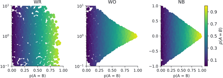
Samples of win rate statistics plotted against $p(A=B)$. As the number of ties increases, $\mathtt{WO}$ and $\mathtt{NB}$ tend to their null effect value, whereas WR is unaffected.
$\mathtt{WR}$ is a relative metric, comparing only two quantities against each other without taking into account the whole sample. $\mathtt{NB}$ and $\mathtt{WO}$ are absolute metrics, which do take the entire sample space into account. Hardy et al. [6] argue that relative measures inflate the difference between systems, and should only be reported alongside absolute metrics.
In general, $\mathtt{WR}$ will always be greater than or equal to $\mathtt{WO}$. How steeply $\mathtt{WR}$ deviates from $\mathtt{WO}$ is determined by the probability of ties. You can clearly see this in the figure below, where $\mathtt{WR}$ and $\mathtt{WO}$ from the same sample are plotted against each other.
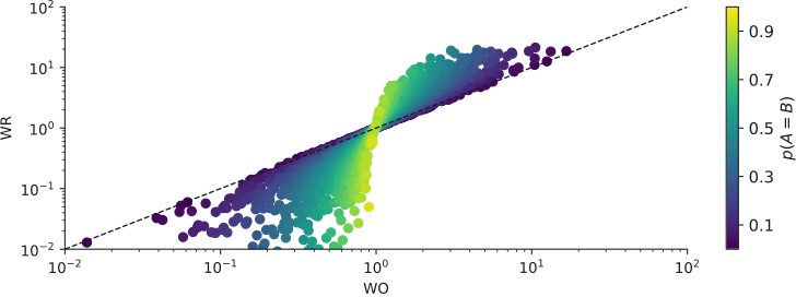
Samples of $\mathtt{WO}$ plotted against $\mathtt{WR}$. Color denotes $p(A=B)$, and the dashed diagonal line gives 1-1 correspondence.
Both $\mathtt{WR}$ and $\mathtt{NB}$ are asymptotically normally distributed. While $\mathtt{WO}$ is not, due to it being an odds ratio, its logarithm $\log\mathtt{WO}$ is also asymptotically normally distributed
If system A stochastically dominates system B, i.e., $p(B\succ A)=0$, $\mathtt{WR}$ is undefined, while $\mathtt{NB}$ and $\mathtt{WO}$ are well-defined. Additionally, if system A always wins, i.e., $p(A\succ B)=1$, only $\mathtt{NB}$ is well-defined, and maximal (although this is a particularly uninteresting edge case).


Confidence Intervals
Pocock et al. (2012) [2] note that $\mathtt{WR}$ is asymptotically normally distributed. They suggest that a natural confidence interval would be:
$$\mathtt{WR}_{\text{LB}}, \mathtt{WR}_{\text{UB}}=\mathtt{WR}\pm c^{*}\cdot \left[\frac{\mathtt{WR}(1-\mathtt{WR})}{N_{A\succ B}+N_{B\succ A}}\right]^{\frac{1}{2}}$$where $c^{*}$ is the critical value corresponding to the confidence level (e.g., $1.96$ for a confidence level of $95\%$). This uses Wald’s normal approximation to Binomial proportion intervals.
Matsouaka (2022) [7] discusses core limitations to this approach. Namely, 1) the variance is estimated under the alternative hypothesis, $H_{1}$, rather than the null hypothesis, $H_{0}$, and 2) Wald’s normal approximation is poor, especially for smaller $N$. They empirically show poor coverage of this confidence interval, especially with small $N$.
Matsouaka (2022) [7] instead recommends relying on Donner and Zou’s (2012) [8] Method of Variance Estimates Recovery (MOVER) approach. Briefly, it uses a geometric argument to suggest that the confidence interval for the difference or sum of two estimates (each of which comes with its own confidence interval) is related to the length of the edge connecting the crossed lower and upper bounds of the separate estimands.
I won’t replicate the derivation of the MOVER bounds here, as these are lengthy (although relatively simple to implement programmatically). For $\mathtt{NB}$, the MOVER confidence interval looks like:
$$\begin{align} \mathtt{NB}_{\text{LB}}&=\mathtt{NB}-\sqrt{(p(A\succ B)-p(A\succ B)_{LB})^2+(p(B\succ A)_{UB}-p(B\succ A))^2-2\rho(p(A\succ B)-p(A\succ B)_{LB})(p(B\succ A)_{UB}-p(B\succ A))} \\ \mathtt{NB}_{\text{UB}}&=\mathtt{NB}+\sqrt{(p(A\succ B)_{UB}-p(A\succ B))^2+(p(B\succ A)-p(B\succ A)_{LB})^2-2\rho(p(A\succ B)_{UB}-p(A\succ B))(p(B\succ A)-p(B\succ A)_{LB})} \end{align}$$where $p(A\succ B)_{LB}, p(A\succ B)_{UB}$ are the lower and upper bounds of the win probability estimated using some standard Binomial proportion interval (I suggest Agresti-Coull), $p(B\succ A)_{LB}, p(B\succ A)_{UB}$ idem but for the loss probability, and $\rho$ is a correlation coefficient between the win and loss probabilities.
Using the earlier provided relations between $\mathtt{NB}$ and $\mathtt{WR}$/$\mathtt{WO}$, their respective CI bounds can also be found after appropriate transformations.
Test Statistic
Besides confidence intervals for the various paired win rate statistics, it would be useful to have an intuitive test statistic which can output a $p$-value. This has been done for $\mathtt{WR}$ by both Pocock et al. and Matsouaka. The Matsouaka test statistic is defined as:
$$Z=\frac{p(A\succ B)-p(B\succ A)}{\sqrt{\mathtt{var}[p(A\succ B)-p(B\succ A)|H_{0}]}}$$where $\mathtt{var}[p(A\succ B)-p(B\succ A)|H_{0}]$ is the variance of $\mathtt{NB}$ under the null hypothesis, defined as $(p(A\succ B)+p(B\succ A))/N$, giving a closed form estimate for $Z$ as:
$$\hat{Z}=\frac{N_{A\succ B}-N_{B\succ A}}{\sqrt{N_{A\succ B}+N_ {B\succ A}}}$$This happens to match McNemar’s test statistic for paired designs, and according to Matsouaka matches “the asymptotic uniformly most powerful nonrandomized test for a nonparametric sign test in the presence of ties.”
Unlike Pocock et al. [2]’s test statistic, Matsouaka [7]’s has type I errors near the desired significance level even for small sample sizes, while having slightly less power (i.e., it is more conservative).
While Matsouaka [7] notes that their approach cannot be applied to derive tests for $\mathtt{WO}$ or $\mathtt{NB}$, Dong et al. (2023) [5] show that this $Z$ statistic is approximately equivalent for all discussed win rate statistics. As such, it probably serves as a good test statistic for all win rate statistics.
Bayesian Approaches
Besides these frequentist approaches, we can also fit a small Bayesian model to this data. Specifically, we can treat each win, loss or tie as samples from a Dirichlet-Categorical distribution. This exact model was already presented by Goutte & Gaussier (2005) [9] for the analysis of information retrieval systems.
Symbolically, this would look like:
$$\tilde{p}(A\succ B), \tilde{p}(B\succ A),\tilde{p}(A=B)\sim\mathtt{Dirichlet}(\alpha_{A\succ B}+N_{A\succ B}, \alpha_{B\succ A}+N_{B\succ A}, \alpha_{A=B}+N_{A=B})$$where $\tilde{p}$ are various sampled probabilities, and $\alpha$ are pseudo-count prior parameters. Then, rather than having to infer the asymptotic sampling distribution of various win rate statistics, we can access their posteriors directly by transforming the win, loss and tie probability samples. Essentially, this trades mathematical rigor for compute, but since the latter is cheaper than the former in the 21st century, this is a reasonable trade-off.
To perform significance testing, we can remain in a Bayesian framework by utilizing the probability of direction and the Region of Practical Equivalence (RoPE) ([10], [11], [12]). For example, to compute the probability of direction (the Bayesian $p$ value) for Matsouaka [7]’s test statistic:
$$\begin{aligned} p_{\text{dir}}(Z)&=\frac{1}{K}\sum_{j=1}^{K}\mathbb{1}\left[\tilde{Z}>0\right] \\ \tilde{Z}_{j}&=\frac{\tilde{p}(A\succ B)_{j}-\tilde{p}(B\succ A)_{j}}{(\tilde{p}(A\succ B)_{j}+\tilde{p}(B\succ A)_{j})^{\frac{1}{2}}N^{-\frac{1}{2}}} \end{aligned}$$where $K$ is the total number of samples from the Dirichlet model, indexed by $j$.
Case Study
I wrote a small Python library, prob_wins which computes the discussed win rate statistics from two vectors of paired results, and provides statistical inference from both the Frequentist and Bayesian frameworks. To showcase it, and give a feel for the various discussed win rate statistics, I thought I’d present a small case study.
EvalEval’s Every Eval Ever datastore contains sample level evaluation of many LLMs on many benchmark datasets. Let’s say we want to test whether llama-3.3-70b-instruct is better than its predecessor (llama-3.2-90b-vision-instruct) on HellaSwag.
Overall, both models are quite good:
            Baseline
Model      N       Y
      +--------+--------+
    N |  2.00% | 14.86% |
      +--------+--------+
    Y | 10.20% | 72.95% |
      +--------+--------+
In only 2% of cases do both models make a mistake, and in 73% of cases, both models are correct. It’s the cases where they differ which is most interesting, however.
We can use prob_wins to quickly estimate various win rate statistics to express precisely how large the difference in win rates is for the two models.
1
2import prob_wins
3pairwise_comparison_results = prob_wins.compare_paired_win_rates_frequentist(
4    results=eval_results_llama33_70b,
5    baseline_results=eval_results_llama32_90b,
6    confidence_level=0.95,
7)
This returns an object containing the following statistics:
| Statistic | Value | 95%CI | Statistic | Value | 95%CI |
|---|---|---|---|---|---|
| $p(A\succ B)$ | 0.1486 | [0.1418, 0.1557] | WR | 1.4570 | [1.3456, 1.5777] |
| $p(B\succ A)$ | 0.1020 | [0.0962, 0.1080] | WO | 1.0978 | [1.0765, 1.1194] |
| $p(A=B)$ | 0.7495 | [0.7409, 0.7578] | NB | 0.0466 | [0.0369, 0.0564] |
From this, we may conclude that the probability of a win is between $\approx 0.04-0.6$ higher than a loss, or that its $\approx 10\%$ more likely to encounter a win or tie rather than a loss or tie. But is this difference statistically significant given the size of Hellaswag?
The $Z$ statistic is $9.33$, meaning that the difference is roughly $9$ times larger than the pairwise standard error. This gives a one-sided p value ($H_{1}=A\succ B$) of $5.28e-21$; we may safely reject the null hypothesis, the difference is clearly statistically significant.
What about from a Bayesian perspective? We can run a similar bit of code to achieve the same result. Note the additional parameters in the signature to set the RNG seed, the Dirichlet prior hyperparameters, the number of samples to draw, and finally, the ROPE boundaries.
1pairwise_comparison_results_bayesian = prob_wins.compare_paired_win_rates_bayesian(
2    results=model_2_eval_results_paired,
3    baseline_results=model_1_eval_results_paired,
4    seed=0,
5    prior_strategy="ones",
6    num_samples=100000,
7    min_sig_diff=2.00,
8)
The quantities in the output object are awfully close to those from the Frequentist analysis.
| Statistic | Median | 95%HDI | Statistic | Median | 95%HDI |
|---|---|---|---|---|---|
| $p(A\succ B)$ | 0.1486 | [0.1415, 0.1555] | WR | 1.4569 | [1.3455, 1.5751] |
| $p(B\succ A)$ | 0.1020 | [0.0961, 0.1079] | WO | 1.0978 | [1.0766, 1.1195] |
| $p(A=B)$ | 0.7493 | [0.7408, 0.7578] | NB | 0.0466 | [0.0370, 0.0565] |
While not necessarily exciting, it does validate the derived bounds for the Frequentist statistics. The $Z$ test statistic is similarly distributed ($Z=9.33~~[7.37, 11.23]$, median [HDI]) as well. Overall, at $1e+5$ samples, this gives a $100\%$ probability that the difference is statistically significant, and similarly, a $100\%$ probability that this difference falls outside the ROPE.
In other words, we can be pretty sure that llama-3.3-70b-instruct is the better model on Hellaswag.
Multiple Comparisons
So far, the discussion has focused on the specific case of pairwise comparisons. When constructing leaderboards (e.g., Chatbot Arena), we want to see how a system compares relative to all other evaluated systems. While you could apply pairwise win rate comparisons to all combinations of models, this quickly becomes impossible to read and suffers from rapidly escalating family-wise error rates.
In those cases, Bradley-Terry or Elo rating models are popular alternatives. These express the probability of system A winning using a specific model:
$$p(A\succ B)=\sigma(r(y_{A}|x)-r(y_{B}|x))$$This is a particularly deep topic, receiving much attention from the human preference learning field. Extensions incorporating ties or rating uncertainty have been proposed. Fully Bayesian alternatives also exist, and are increasingly popular.
My main point of criticism of these models is that an Elo rating is inherently uninterpretable. It merely suggests that given a difference of ratings between two systems, then there’s a particular probability of one system being preferred over the other. It does not answer whether this difference is significant or not.
It is also a predictive model. Its main purpose is to predict the probability of a win given two comparisons which have not been tested against each other. In theory, if we evaluate a system against an infinite amount of terrible alternatives, we can inflate its score far beyond what is warranted, especially given that it’s never been evaluated against a comparable system 1.
Conclusion & Recommendations
Evaluating LLMs is hard, and it’s only getting harder as we apply these models in domains where it’s difficult to asign a single ground truth value to any input. Moving away from evaluation metrics to general purpose paired win rates simplifies the evaluation procedure, but currently comes without statistical significance testing.
Luckily, with very little work we can compute sensible effect size statistics with closed form confidence bounds. We can additionally derive a hypothesis test, which has large amounts of prior work backing it up. Hopefully, these findings help regularize machine learning findings.
The prob_wins package can be downloaded from PyPi!
References
- Q. Li, Y. Zhu, Y. Zhao, C. Danzeng, D. Wang, R. Jiang, F. Chen, X. Lin, L. Hu, and Y. Wang,
The win ratio in contemporary clinical trials: growing adoption and interpretation challenges—a meta-epidemiological study,
Journal of Clinical Epidemiology, vol. 196, p. 112315, 2026. doi:10.1016/j.jclinepi.2026.112315 - S. Pocock, C. Ariti, T. Collier, and D. Wang,
The win ratio: a new approach to the analysis of composite endpoints in clinical trials based on clinical priorities,
European Heart Journal, vol. 33, no. 2, p. 176–182, 2012. doi:10.1093/eurheartj/ehr352 - E. Brunner, M. Vandemeulebroecke, and T. Mütze,
Win odds: an adaptation of the win ratio to include ties,
Statistics in Medicine, vol. 40, no. 14, p. 3367–3384, 2021. doi:10.1002/sim.8967 - G. Noether,
Sample Size Determination for Some Common Nonparametric Tests,
Journal of the American Statistical Association, vol. 82, no. 398, p. 645–647, 1987. doi:10.2307/2289477 - G. Dong, D. Hoaglin, B. Huang, Y. Cui, D. Wang, Y. Cheng, and M. Gamalo-Siebers,
The stratified win statistics (win ratio, win odds, and net benefit),
Pharmaceutical Statistics, vol. 22, no. 4, p. 748–756, 2023. doi:10.1002/pst.2293 - M. Hardy, S. Ong, and D. Paterson,
The win ratio should be complemented by other win statistics to provide a comprehensive picture of relative and absolute treatment effects: the case study of the REPRIEVE trial,
Clinical infectious diseases, vol. 82, no. 2, p. e413–e414, 2026. doi:10.1093/cid/ciaf587 - R. Matsouaka,
Robust statistical inference for matched win statistics,
Statistical Methods in Medical Research, vol. 31, no. 8, p. 1423–1438, 2022. doi:10.1177/09622802221090761 - A. Donner and G. Zou,
Closed-form confidence intervals for functions of the normal mean and standard deviation,
Statistical Methods in Medical Research, vol. 21, no. 4, p. 347–359, 2012. doi:10.1177/0962280210383082 - C. Goutte and E. Gaussier,
A Probabilistic Interpretation of Precision, Recall and F -score, with Implication for Evaluation,
2005. - J. Kruschke,
Bayesian estimation supersedes the t test.,
Journal of Experimental Psychology: General, vol. 142, no. 2, p. 573–603, 2013. doi:10.1037/a0029146 - J. Kruschke and T. Liddell,
The Bayesian New Statistics: Hypothesis testing, estimation, meta-analysis, and power analysis from a Bayesian perspective,
Psychonomic Bulletin & Review, vol. 25, no. 1, p. 178–206, 2018. doi:10.3758/s13423-016-1221-4 - D. Makowski, M. Ben-Shachar, S. Chen, and D. Lüdecke,
Indices of Effect Existence and Significance in the Bayesian Framework,
Frontiers in Psychology, vol. 10, 2019. doi:10.3389/fpsyg.2019.02767
Changelog
[2026-07-06] First draftthere are more issues with these style models, or rather their application. That is not to say that I’m not a fan of the Elo rating system; learning about it is what led me down a statistics/machine-learning rabbit hole that I will likely never escape ↩︎