Priors#
tldr: few classes, use 1 as a prior value. Many classes and enough data, use 0.
In prob_conf_mat, we use a probabilistic model of the confusion matrix to sample synthetic confusion matrices. Specifically, we use the product of several Dirichlet-Categorical distributions to sample counterfactuals. These distributions are constrained by the data in the true confusion matrix, and in Bayesian statistics would be called a posterior distribution; the distribution that arises when we combine knowledge we know a priori with evidence.
The knowledge we know a priori is summarized as a prior distribution, and represents the knowledge contained in the model before any evidence is taken into account.
In prob_conf_mat, each experiment is equipped with two priors:
- the
prevalence_prior(\(\text{num_classes}\)), which tells us how often we expect each condition to appear in the data - the
confusion_prior(\(\text{num_classes}\times \text{num_classes}\)), which tells us how often we expect the model predict each class, given the ground-truth condition
These can be useful to inject external knowledge into our analyses. For example, if we know that a certain disease is present in 1% of the population, but our disease detector is evaluated on balanced data (50/50) then we can use the prior distribution to take the true disease prevalence into account. As a result, our performance metrics automatically shift to reflect performance under the true occurrence rate.
Most of the time, however, we don't have any prior information. In this case, we want to choose a prior that has minimal effect on our analysis, while still regularizing the posterior a little. In Bayesian statistics terms, we want an uninformative prior. What does or does not constitute an uninformative prior is a matter of continued debate, but values of all 0.0, 0.5 or 1.0 are common choices for the Beta-Binomial model (the univariate special case of the Dirichlet-Categorical model).
To set priors in prob_conf_mat, you can pass either:
- a
strcorresponding to a registered prior strategy - a scalar numeric (
float | int), in which all parameters will be set to that value - an
ArrayLikeof numerics, in which the prior parameters are copied from the passedArrayLike
See prob_conf_mat.stats.dirichlet_distribution.dirichlet_prior for more information.
Effect of Uninformative Priors on Metric Samples#
It is a feature of the confusion matrix model that the priors of the metric distributions are generally not flat, despite uninformative priors being used. Intuitively, this makes sense. A model that is equally likely to predict any class, regardless of the ground-truth condition, is likely not a good model.
This can be seen in the following figure. It displays the empirical distribution of some metrics given a prior of all 1s, across various different number of classes.
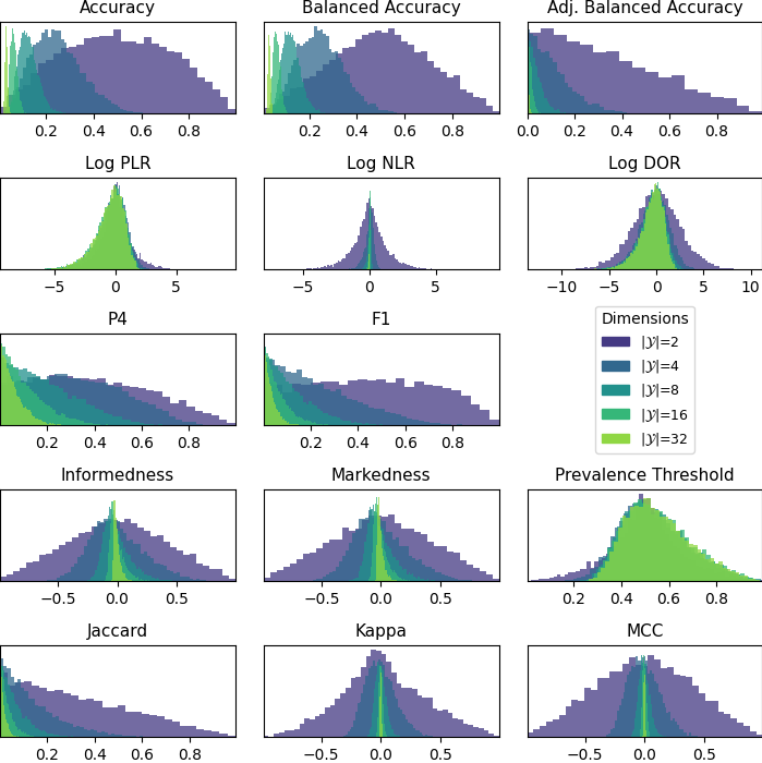
In all cases, the distributions are centered around the value corresponding to random performance, although this differs for each metric. As, the number of classes increases, however, most of the prior distributions become increasingly narrow. This means, even an uninformative prior can have undue influence on the eventual posterior distribution in higher dimensions.
This is similar to using a prior with a much larger constant value (implying a greater degree of prior information). The following figure shows this:
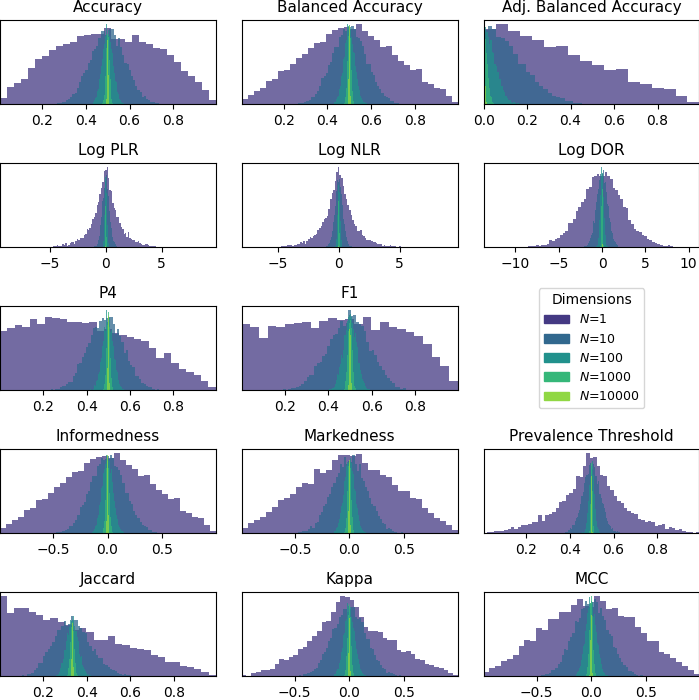
Like before, the metric prior distributions are all centered around the random performance value (the number of classes is held constant at 2), and the priors become more narrow as the prior value (\(N\)) increases.
Creating a truly uninformative prior (i.e., a flat distribution) for each metric is likely not possible with the synthetic confusion matrix sampling procedure bayes_conf_mat uses. For experiments with relatively few classes, we can get away with a standard prior, like the Bayes-Laplace prior of all 1s. For experiments with large number of classes, however, any value we choose will lead to a narrow and peaked metric prior, and will have a large effect on our analysis. Hence, we recommend the following guidelines:
- If you have very few classes (\(<4\)), set prior parameters like 0.5 or 1. These will regularize the posterior metric distributions a bit, but not by an undue amount
- If you have many classes, and a lot of data, use 0 as your prior value. The posterior will not be regularized, but we expect the data to dominate anyway
- If you have many classes, but only a small amount of data, either set a small prior value, or use 0 and interpret your analysis with a grain of salt